Univariate amputation

This example demonstrates different ways to amputate a dataset in an univariate manner.

# Author: G. Lemaitre
# License: BSD 3 clause

import sklearn
import seaborn as sns

sklearn.set_config(display="diagram")
sns.set_context("poster")

Let’s create a synthetic dataset composed of 10 features. The idea will be to amputate some of the observations with different strategies.

import pandas as pd
from sklearn.datasets import make_classification

X, y = make_classification(n_samples=10_000, n_features=10, random_state=42)

feature_names = [f"Features #{i}" for i in range(X.shape[1])]
X = pd.DataFrame(X, columns=feature_names)

Missing completely at random (MCAR)

We will show how to amputate the dataset using a MCAR strategy. Thus, we will amputate 3 given features randomly selected.

import numpy as np

rng = np.random.default_rng(42)
n_features_with_missing_values = 3
features_with_missing_values = rng.choice(
    feature_names, size=n_features_with_missing_values, replace=False
)

Now that we selected the features to be amputated, we can create an transformer that can amputate the dataset.

from ampute import UnivariateAmputer

amputer = UnivariateAmputer(
    strategy="mcar",
    subset=features_with_missing_values,
    ratio_missingness=[0.2, 0.3, 0.4],
)

If we want to amputate the full-dataset, we can directly use the instance of UnivariateAmputer as a callable.

X_missing = amputer(X)
X_missing.head()

	Features #0	Features #1	Features #2	Features #3	Features #4	Features #5	Features #6	Features #7	Features #8	Features #9
0	NaN	0.357385	-0.503931	0.935066	0.647981	-0.050796	-1.933989	2.081684	0.041266	-0.258298
1	1.283905	1.109459	-0.908953	1.006586	0.492219	1.107295	1.243526	-0.172200	1.150359	0.147744
2	-0.966476	-0.593314	0.458020	1.032323	1.283685	-0.317640	1.499045	0.434477	0.423678	1.251380
3	2.429309	-1.306530	-1.869925	3.092164	2.028800	-0.879635	NaN	-0.101213	-1.624066	NaN
4	NaN	0.078464	0.705181	0.224765	0.618707	1.534946	NaN	2.325055	0.495505	0.538133

We can quickly check if we get the expected amount of missing values for the amputated features.

import matplotlib.pyplot as plt

ax = X_missing[features_with_missing_values].isna().mean().plot.barh()
ax.set_title("Proportion of missing values")
plt.tight_layout()

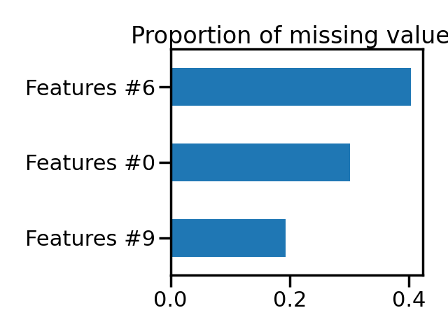
Thus we see that we have the expected amount of missing values for the selected features.

Now, we can show how to amputate a dataset as part of the scikit-learn Pipeline.

from sklearn.impute import SimpleImputer
from sklearn.preprocessing import StandardScaler
from sklearn.linear_model import LogisticRegression
from sklearn.pipeline import make_pipeline
from sklearn.model_selection import cross_val_score
from sklearn.model_selection import ShuffleSplit

model = make_pipeline(
    amputer,
    StandardScaler(),
    SimpleImputer(strategy="mean"),
    LogisticRegression(),
)
model

Pipeline

Pipeline(steps=[('univariateamputer',
                 UnivariateAmputer(ratio_missingness=[0.2, 0.3, 0.4],
                                   subset=array(['Features #9', 'Features #0', 'Features #6'], dtype='

UnivariateAmputer

UnivariateAmputer(ratio_missingness=[0.2, 0.3, 0.4],
                  subset=array(['Features #9', 'Features #0', 'Features #6'], dtype='

StandardScaler

StandardScaler()

SimpleImputer

SimpleImputer()

LogisticRegression

LogisticRegression()

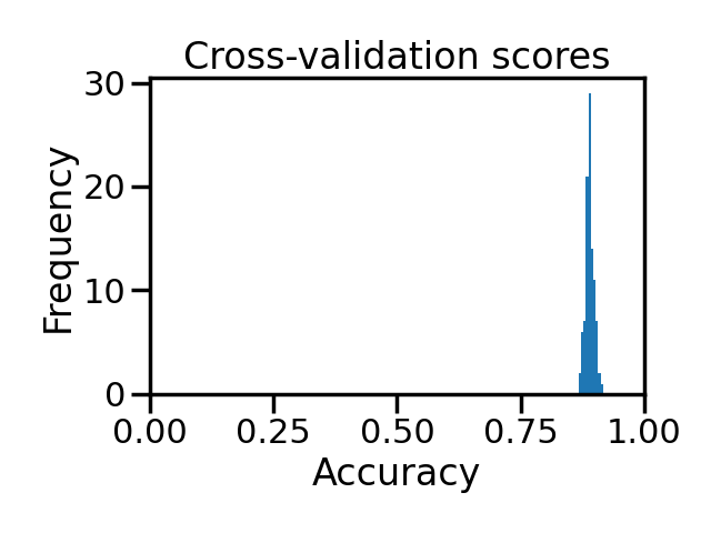
Now that we have our pipeline, we can evaluate it as usual with any cross-validation tools provided by scikit-learn.

n_folds = 100
cv = ShuffleSplit(n_splits=n_folds, random_state=42)
results = pd.Series(
    cross_val_score(model, X, y, cv=cv, n_jobs=2),
    index=[f"Fold #{i}" for i in range(n_folds)],
)

ax = results.plot.hist()
ax.set_xlim([0, 1])
ax.set_xlabel("Accuracy")
ax.set_title("Cross-validation scores")
plt.tight_layout()

previous

Examples

next

Release history